VLOOKUP is the most popular and useful lookup function in Excel and Google Sheets, But the VLOOKUP function has some limitations and due to those limitations, most of the users face VLOOKUP Value #NA error. This article will help you to fix this error easily.
How To Fix VLOOKUP #NA Error
VLOOKUP #NA (Not Available) error message occurs when Excel can not find its lookup value. There are several ways to fix this error easily.
You can use the following ways to fix this error.
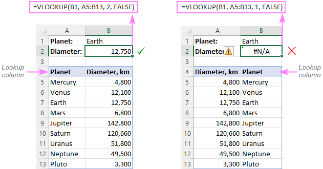
The Lookup Column must be at the Leftmost Column of the Table Array
If the Lookup column is not at the leftmost column of the table array, Then it will show a VLOOKUP #NA error message instead of the lookup value. You can fix this error by just shifting the Lookup column to the leftmost side of the Table array.
Format Cells as Numbers
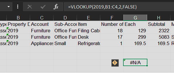
If the table cells are formatted as text, the value will treated as straight text whether it’s a number, date, or other data type. You can fix this by reformatting the cells as numeric data type.
Remove Extra Spaces
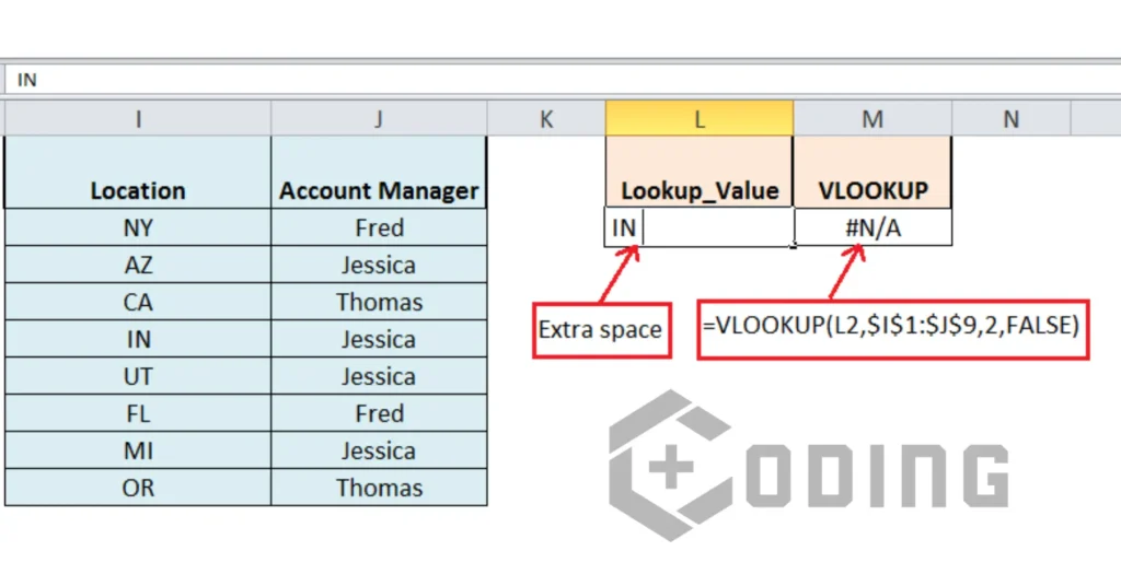
Excel and Spreadsheets gotcha leads to trailing spaces in data items. Since VLOOKUP searches for an exact match and if data have extra spaces at the front or end of data, it will lead to VLOOKUP #NA error. You can remove extra spaces to fix this error.
Apply LEN Excel Formula
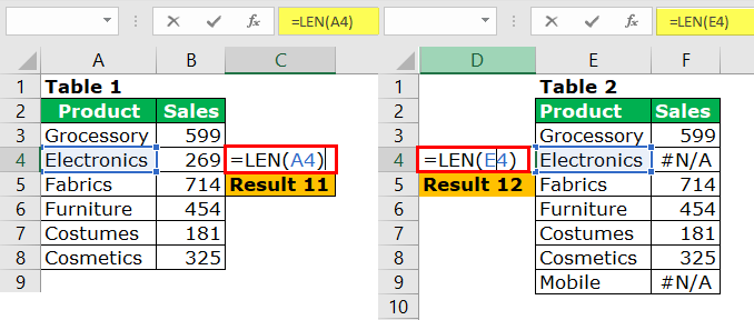
You can use the LEN Excel formula to detect extra spaces and delete them easily. In C4, The LEN function is applied to find the number of characters in A4. Similarly, you can use the LEN function in D4 to find the count of characters in cell E4.
If the Count is different, it means there are extra spaces which can cause VLOOKUP #NA error, You can resolve this by deleting extra spaces.
These are 4 common ways to fix VLOOKUP #NA error, by using this, you can easily fix this error.
Read More: QR Code Not Working on iPhone

